Finding zeros of data using QSoas

QSoas does not provide by default commands to detect zeros of data, and the reason for that is that it is simple, using the integrate command to convert this problem into a peak-finding problem, which can be solved using the find-peaks command. Here is that strategy applied to determining the zeros of the 0-th order bessel function:

QSoas> generate-buffer -10 10 bessel_j0(x) /samples=100001
QSoas> integrate
Current buffer now is: 'generated_int.dat'
QSoas> find-peaks
Found 6 peaks
buffer what x y index width left_width right_width
generated_int.dat min -8.6538 -0.201157042341714 6731 1.7798 0.905999999999999 0.873800000000001
generated_int.dat max -5.52 0.398165469321319 22400 2.2854 1.1862 1.0992
generated_int.dat min -2.4048 -0.403288737672291 37976 1.8232 0.973 0.850199999999999
generated_int.dat max 2.4048 2.53731134529594 62024 nan 2.2026 nan
generated_int.dat min 5.52 1.73585713830231 77600 nan 5.7198 nan
generated_int.dat max 8.6538 2.33517964996535 93269 nan 8.5532 nan

Compare that with the values given on Mathematica's website. This strategy is reasonably resistant to noise, since integration decreases high-frequency noise, but you may have to play with the /window option to find-peaks to avoid detecting the same zero (peak) several times.

Hopefully, I'll come back with more regular postings of tips and tricks !

QSoas version 2.0 is out / QSoas paper

I thought it would come before that, but I've finally gotten around releasing version 2.0 of my data analysis program, QSoas !

It provides significant improvements to the fit interface, in particular for multi-buffer fits, with a “Multi” fit engine that performs very well for large multibuffer fits, a spreadsheet editor for fit parameters, and more usability improvements. It also features the definition of fits with distribution of values of one of the fit parameter, and new built-in fits. In addition, QSoas version 2.0 features new commands to derive data, to flag buffers and handle large multi-column datasets, and improvements of existing commands. The full list of changes since version 1.0 can be found there.

As before, you can download the source code from our website, and purchase the pre-built binaries following the links from that page too.

In addition, I am glad to announce that QSoas is now described in a recent publication, Fourmond, Anal. Chem., 2016, 88, 5050-5052. Please cite this publication if you used QSoas to process your data.

Release 0.14.1 of ctioga2

With the (relatively, sorry) recent switch to ruby2.3 as default Ruby version, I realized that my plotting program ctioga2 crashed with ruby 2.3 (due to a rather ugly lazy hack). I have just fixed this in release 0.14.1. Update as usual with:

~ gem update ctioga2

If you're not using Ruby 2.3, you probably don't need to update soon, though. Enjoy !

Release of ctioga2 version 0.14

The day has finally come again to release a new version of my plotting program, ctioga2. Version 0.14 features, among others:

• a new binner, useful to make histograms;
• a command to hide elements already presents, that can be very useful to make animations;
• a whole set of functionalities to make it easier to draw complex grids, including easy ways to style grid elements and a way to switch to the next grid element (picture);
• a whole series of command-file functions to obtain informations about loaded datasets;
• a way to draw legends separately by hand;
• and more, including bugfixes, better error reporting, such as when some of the numbers are infinite, and much much faster debug output.

As usual, the best way to update the package is running:

~ gem update ctioga2

An updated Debian package should find its way to the archive later on today. Have fun !

QSoas tips and tricks: better baselines using the "save points" feature

During data processing in our team, we often subtract plain polynomial baselines to our data, drawn by hand using the b command. Note that this is legitimate because we know that the signal we are looking for quickly drops to 0 outside a given range. The usual workflow is to just load the data, use b to draw a baseline and subtract it, and then have further fun with the baseline-subtracted data. This was the only possibility in the old SOAS. However, I don't like so much this kind of workflow, because such a baseline is arbitrary, and once it's subtracted, it's hard to reassess the baseline afterwards.

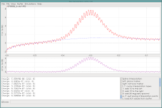
This is why I've designed a better way in QSoas: when you are done creating a baseline, push p: this exits pushing only the interpolation nodes:

Above, the baseline subtraction interface, and below, the resulting nodes:

The nodes can be reloaded by hitting uppercase L from within b and giving a buffer number (admittedly, the interface as of now isn't that good, I'll have to work on it). Alternatively, you can greenerate the baseline by using interpolate, and then further subtract it using S:

QSoas> interpolate 1 0

where 1 is the original buffer (in fact, only its X values will be used, so you don't have to use the same buffer) and 0 is the buffer containing the interpolation nodes. Saving only the interpolation nodes makes it possible to reedit the baseline easily, and regenerate the baseline-subtracted data using a script. This is my favorite approach, because I like to be able to trace every single step from the raw data to processed data. Another neat feature is that, from within b, you can reload only the X values of nodes using lowercase l (and giving buffer number): the Y values are computed as if you had clicked at the corresponding positions. This is very useful is you have a whole series of similar baselines to make: most often, you won't even need manual adjustment to get a good baseline. I hope you'll find this tip useful !

Making oprofile work again with recent kernels

I've been using oprofile for profiling programs for a while now (and especially QSoas, because it doesn't require specific compilation options, and doesn't make your program run much more slowly (like valgrind does, which can also be used to some extent for profiling). It's a pity the Debian package was dropped long ago, but the ubuntu packages work out of the box on Debian. But, today, while trying to see what takes so long in some fits I'm running, here's what I get:

~ operf QSoas
Unexpected error running operf: Permission denied

Looking further using strace, I could see that what was not working was the first call to perf_event_open.
It took me quite a long time to understand why it stopped working and how to get it working again, so here's for those of you who googled the error and couldn't find any answer (including me, who will probably have forgotten the anwser in a couple of months). The reason behing the change is that, for security reason, non-privileged users do not have the necessary privileges since Debian kernel 4.1.3-1; here's the relevant bit from the changelog:

  * security: Apply and enable GRKERNSEC_PERF_HARDEN feature from Grsecurity,
    disabling use of perf_event_open() by unprivileged users by default
    (sysctl: kernel.perf_event_paranoid)

The solution is simple, just run as root:

~ sysctl kernel.perf_event_paranoid=1

(the default value seems to be 3, for now). Hope it helps !

QSoas tips and tricks: using the fit interface to explore parameters to a function

As I said before, one of the very strong points of QSoas, my data analysis software, is its fitting capacities, and its fitting interface. Today, as a first post in a series of tips and tricks about QSoas, I will show you that the fit interface can also be used for a quick exploration of the effect of parameters on a given function. For that, I have chosen a simple system, the Van der Pol oscillator. The differential equation can be written for QSoas in the following form (in a file named vanderpol.ode):

x = x_0
y = dx_0

d_x = y
d_y = mu * (1 - x**2) * y - x

Note the blank line between the initial conditions and the expression for the derivatives. This is the representation of the form using y as the derivative of x. The integration variable in QSoas is the time t. You can learn more about how to specify differential equations in QSoas from the manual. The game is now simply to use fit-ode to launch the fit interface, but before that, one needs data to serve as a template, generated using generate-buffer:

QSoas> generate-buffer 0 100 1
QSoas> fit-ode vanderpol.ode

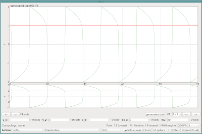
Now, the fit interface looks like this:

You can play around with the parameters, and in particular the value of mu... For every modification, hit the Update button, or just Ctrl+U, to see the effect. For data you'd wish to take a closer look at, use the Push current to stack action from the Data... menu, which creates new buffers on the stack. A nice thing is that QSoas keeps the fit parameters as meta-data, which you can see later on using show:

See the values of mu in the terminal above ?

This feature of QSoas makes it easy to quickly explore the effect of the parameters of a model on the shape of the resulting curve. I have used that very heavily in my research, I hope others will find it useful too. Enjoy !

Ghost in the machine: faint remanence of screen contents across reboots in a Macbook pro retina

As was noted a few times before, I happen to own a Macbook Pro Retina laptop I mostly use under Linux. I had noticed from time to time weird mixes between two screens, i.e. I would be looking at a website, but, in some areas with uniform colors, I would see faint traces of other windows currently opened on another screen. These faint traces would not show up in a screenshot. It never really bothered me, and I attributed that to a weird specificity of the mac hardware (they often do that) that was not well handled by the nouveau driver, so I had simply dismissed that. Until, one day, I switch off the computer, switch back on, boot to MacOS and see this as a boot screen:

Here is a close-up view of the top-left corner of the screen:

If you look carefully, you can still see the contents of the page I was browsing just before switching off the computer ! So this problem is not Linux-specific, it also affects MacOS... To be honest, I don't have a clue about what's happening here, but it has to be a serious hardware malfunction. How can two video memory regions be composed upon display without the computer asking explicitly for it ? Why does that problem survives a reboot ? I mean, someone switches on my computer and can see the last thing I did on it ? I could actually read the address line without difficulty, although you'll have to take my word for it, since the picture does not show it that well. That's scary...