QSoas tips and tricks: better baselines using the "save points" feature

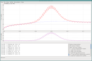
During data processing in our team, we often subtract plain polynomial baselines to our data, drawn by hand using the b command. Note that this is legitimate because we know that the signal we are looking for quickly drops to 0 outside a given range. The usual workflow is to just load the data, use b to draw a baseline and subtract it, and then have further fun with the baseline-subtracted data. This was the only possibility in the old SOAS. However, I don't like so much this kind of workflow, because such a baseline is arbitrary, and once it's subtracted, it's hard to reassess the baseline afterwards.

This is why I've designed a better way in QSoas: when you are done creating a baseline, push p: this exits pushing only the interpolation nodes:

Above, the baseline subtraction interface, and below, the resulting nodes:

The nodes can be reloaded by hitting uppercase L from within b and giving a buffer number (admittedly, the interface as of now isn't that good, I'll have to work on it). Alternatively, you can greenerate the baseline by using interpolate, and then further subtract it using S:

QSoas> interpolate 1 0

where 1 is the original buffer (in fact, only its X values will be used, so you don't have to use the same buffer) and 0 is the buffer containing the interpolation nodes. Saving only the interpolation nodes makes it possible to reedit the baseline easily, and regenerate the baseline-subtracted data using a script. This is my favorite approach, because I like to be able to trace every single step from the raw data to processed data. Another neat feature is that, from within b, you can reload only the X values of nodes using lowercase l (and giving buffer number): the Y values are computed as if you had clicked at the corresponding positions. This is very useful is you have a whole series of similar baselines to make: most often, you won't even need manual adjustment to get a good baseline. I hope you'll find this tip useful !