QSoas tips and tricks: using the fit interface to explore parameters to a function

As I said before, one of the very strong points of QSoas, my data analysis software, is its fitting capacities, and its fitting interface. Today, as a first post in a series of tips and tricks about QSoas, I will show you that the fit interface can also be used for a quick exploration of the effect of parameters on a given function. For that, I have chosen a simple system, the Van der Pol oscillator. The differential equation can be written for QSoas in the following form (in a file named vanderpol.ode):

x = x_0
y = dx_0

d_x = y
d_y = mu * (1 - x**2) * y - x

Note the blank line between the initial conditions and the expression for the derivatives. This is the representation of the form using y as the derivative of x. The integration variable in QSoas is the time t. You can learn more about how to specify differential equations in QSoas from the manual. The game is now simply to use fit-ode to launch the fit interface, but before that, one needs data to serve as a template, generated using generate-buffer:

QSoas> generate-buffer 0 100 1
QSoas> fit-ode vanderpol.ode

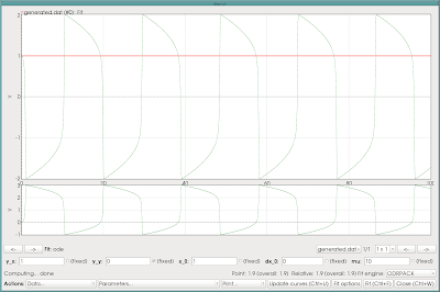
Now, the fit interface looks like this:

You can play around with the parameters, and in particular the value of mu... For every modification, hit the Update button, or just Ctrl+U, to see the effect. For data you'd wish to take a closer look at, use the Push current to stack action from the Data... menu, which creates new buffers on the stack. A nice thing is that QSoas keeps the fit parameters as meta-data, which you can see later on using show:

See the values of mu in the terminal above ?

This feature of QSoas makes it easy to quickly explore the effect of the parameters of a model on the shape of the resulting curve. I have used that very heavily in my research, I hope others will find it useful too. Enjoy !

Ghost in the machine: faint remanence of screen contents across reboots in a Macbook pro retina

As was noted a few times before, I happen to own a Macbook Pro Retina laptop I mostly use under Linux. I had noticed from time to time weird mixes between two screens, i.e. I would be looking at a website, but, in some areas with uniform colors, I would see faint traces of other windows currently opened on another screen. These faint traces would not show up in a screenshot. It never really bothered me, and I attributed that to a weird specificity of the mac hardware (they often do that) that was not well handled by the nouveau driver, so I had simply dismissed that. Until, one day, I switch off the computer, switch back on, boot to MacOS and see this as a boot screen:

Here is a close-up view of the top-left corner of the screen:

If you look carefully, you can still see the contents of the page I was browsing just before switching off the computer ! So this problem is not Linux-specific, it also affects MacOS... To be honest, I don't have a clue about what's happening here, but it has to be a serious hardware malfunction. How can two video memory regions be composed upon display without the computer asking explicitly for it ? Why does that problem survives a reboot ? I mean, someone switches on my computer and can see the last thing I did on it ? I could actually read the address line without difficulty, although you'll have to take my word for it, since the picture does not show it that well. That's scary...